Introductory guid to portfolio selection with Python

Introduction

Harry Markowitz introduced modern portfolio theory in his 1952 paper titled Portfolio Selection. He begins by outlining that portfolio selection is a two-step process; firstly, an investor must consider the future performance of the available assets (in terms of both risk and return) and subsequently, a decision can be made about how to construct the portfolio (i.e. how much money to allocate to each asset).

The main objective of constructing a portfolio is to reduce risk without necessarily decreasing expected rate of return. From this, risk and return are the main characteristics of the portfolio, or any financial instrument for that matter. Therefore, optimizing a portfolio is maximizing overall return while minimizing the risk. It is a hard task to do considering the fact that risk and return are positively correlated, meaning that if risk is high, return is high as well.

Return

Buying a financial asset can bring two types of return: dividend or interest payment and capital gain/loss. Therefore, return for the entire single holding period is as follows:

$R = capital gain + dividend yeild = \frac{P_{t}-P_{t-1}+D_{t}}{P_{t-1}}$

However, this calculation doesn’t take into account the length of the period, holding period could be a month or even 10 years. The fact that this return is not annualized makes it hard for us to use it for comparison. For multiple periods, like several years, we can use either mean return or geometric mean return to aggregate the rates of return. Former one calculates overall return by dividing the sum of returns by the number of periods (years). Pretty easy and straightforward. However, this method assumes that the amount invested in the same at the beginning of each period, hence, it doesn’t take into account the compounding of return. This is why geometric mean return is a better representation of portfolio return.

Here we assume that our portfolio is a long-term “buy-hold” portfolio, therefore using geometric mean is more suitable. Please note that using historical returns for calculating expected returns (in our case calculating geometric mean of historical returns and using is as a proxy for expected return) could be inaccurate in some cases!

Risk

Portfolio risk is a chance that the combination of assets or units, within the investments that you own, fail to meet financial objectives. We calculate risk by measuring volatility of the returns using statistical measures such as variance, standard deviation, and covariance. Calculating standard deviation of a single financial asset is pretty straightforward: $\sigma = \sqrt{\frac{1}{N} \sum_{i=1}^N (x_i - \mu)^2}$ .

But when it comes to finding the portfolio’s variance, weighted average of financial assets’ variances will not do the trick because we have to consider correlation between the assets. The general equation goes like this: $\sigma^2 = \sum_{i,j=1}^N w_{i} w_{j} Cov(R_{i} R_{j})$ .

Note that in order to simplify the evaluation, we assume that the returns are normally distributed, therefore can be described by its mean and variance. If this assumption is violated, there would be additional characteristics such as skewness and kurtosis.

Python codes

First, we define two classes as class stock and class portfolio with required functions in each class like the following:

import numpy as np
from scipy import optimize 
import matplotlib as plt

#class Stock takes array of closing prices at the beginning and at the end of the year
#and calculates geometric return and standard deviation
#to simplify the calculation let's assume that there are no dividends
class Stock:
    def __init__(self, prices):
        self.prices = prices

    def annual_returns(self):
        returns = []
        for i in range(0, len(self.prices)-1):
            returns.append((self.prices[i+1]-self.prices[i])/self.prices[i])
        return(returns)
            
    def geometric_return(self, returns):
        return(np.prod([x+1 for x in returns])**(1/len(returns))-1)
    
    def standard_deviation(self, returns):
        mean = sum(returns)/len(returns)
        return(np.sqrt(sum([(x-mean)**2 for x in returns])/len(returns)))

#class portfolio takes matrix of returns for every stock, and array of their weights
class Portfolio:
    def __init__(self, returns):
        self.returns = returns
    
    def portfolio_return(self, weights):
        geo_returns = []
        for i in range(0, len(self.returns)):        
            geo_returns.append(np.prod([x+1 for x in self.returns[i]])**(1/len(self.returns[i]))-1)
        return(sum([a*b for a,b in zip(weights, geo_returns)]))
        #return(geo_returns)

    def portfolio_volatility(self, weights):
        sd_values = []
        for i in self.returns:
            mean = sum(i)/len(i)
            sd_values.append(np.sqrt(sum([(x-mean)**2 for x in i])/len(i)))
        weighted_average = [a*b for a,b in zip(weights, sd_values)]
        corr = np.corrcoef(self.returns)
        values = []
        for j in range(0, len(weighted_average)):
            values.append(sum([weighted_average[j]*weighted_average[x]*corr[j,x] for x in range(0,len(weighted_average))]))
        return(np.sqrt(sum(values)))
        #return(values)

    def optimal_portfolio(self, desired_return):
        bounds = ((0.0, 1.0),) * len(self.returns)
        init = list(np.random.dirichlet(np.ones(len(self.returns)), size= 1)[0])
        optimal_weights = optimize.minimize(self.portfolio_volatility, init, method='SLSQP',
            constraints=({'type': 'eq', 'fun': lambda inputs: 1.0 - np.sum(inputs)},
            {'type': 'eq', 'fun': lambda inputs: desired_return - self.portfolio_return(weights=inputs)}), bounds = bounds)
        return optimal_weights.x

Constructing the portfolio

After we’re done with defining functions for calculation of two main characteristics: return and risk, we shall start constructing the portfolio. I’m using yfinance module to get trading data from Yahoo! Finance.

Let’s assume that we’re considering 9 stocks: Amazon, Apple, Google, Nike, Starbucks, The Southern Company, Intel Corporation, Cisco Systems and MetLife. And let’s extract the historical data on each of those (using stock prices at the end of each year).

import yfinance as yf
import pandas as pd

stocks_to_portfolio = ['AMZN', 'AAPL','GOOGL', 'SBUX','NKE', 'SO', 'INTC', 'CSCO', 'MET']

return_matrix = []
stock_char = []
for i in stocks_to_portfolio:
    stock = yf.Ticker(i)
    stock = stock.history(period='10y')
    data = stock.groupby(stock.index.year).apply(pd.Series.tail,1)
    prices = list(data['Close'])
    stock = Stock(prices)
    stock_char.append([i, stock.geometric_return(stock.annual_returns()), stock.standard_deviation(stock.annual_returns())])
    return_matrix.append(stock.annual_returns())

stock_char

The return and volatility of each one looks something like this:

[['AMZN', 0.3476909048776389, 0.37890285434588206],
 ['AAPL', 0.3039892922984164, 0.3109028924005264],
 ['GOOGL', 0.24696159081269897, 0.24159029975307134],
 ['SBUX', 0.19162712648225866, 0.18047608365432197],
 ['NKE', 0.22665887703919307, 0.18705252088261798],
 ['SO', 0.08510454865390904, 0.16384354149552766],
 ['INTC', 0.11000314509944009, 0.19236852159004345],
 ['CSCO', 0.1661399078846546, 0.13202793819065048],
 ['MET', 0.11810236562383247, 0.23320842196338287]]

Now we generate 10,000 random weights and calculated portfolio return and volatility on each of them.

plot_data = []
n = 0
while n < 10000:
    weight = list(np.random.dirichlet(np.ones(len(return_matrix)), size= 1)[0])
    port = Portfolio(return_matrix)
    plot_data.append([weight, port.portfolio_return(weight), port.portfolio_volatility(weight)])
    n += 1

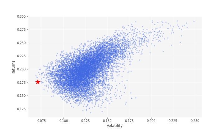
And let’s plot the result. It is safe to assume that given these 9 stocks, the minimum-variance frontier is the set of portfolios along the left border of the point of the following graph.

portfolios  = pd.DataFrame(plot_data)
portfolios = portfolios[[1,2]]
portfolios.columns=['Returns', 'Volatility']
portfolios.plot.scatter(x='Volatility', y='Returns', marker='o', s=10, alpha=0.3, grid=True, figsize=[10,6],color='royalblue')
plt.xlabel('Volatility')
plt.ylabel('Returns')
ax = plt.gca()
ax.set_facecolor('whitesmoke')
plt.show()

Now, we are looking for the portfolio with minimum volatility. Minimum volatilty portfolio is presented in the following graph with a red star.

min_vol_port = portfolios.iloc[portfolios['Volatility'].idxmin()]
min_vol_port

Returns       0.176098
Volatility    0.070633
Name: 1083, dtype: float64

# plotting the minimum volatility portfolio
plt.scatter(min_vol_port[1], min_vol_port[0], color='r', marker='*', s=300)
plt.show()

Sharpe Ratio

The ratio is the average return earned in excess of the risk-free rate per unit of volatility or total risk. Volatility is a measure of the price fluctuations of an asset or portfolio.

The risk-free rate of return is the return on an investment with zero risk, meaning it’s the return investors could expect for taking no risk.

The optimal risky portfolio is the one with the highest Sharpe ratio. The formula for this ratio is: $Sharpe Ratio = \frac{R_{p} - R_{f} }{\sigma_p}$ .

Now we can find optimal risky portfolio. An optimal risky portfolio can be considered as one that has highest Sharpe ratio.

# Finding the optimal risky portfolio

rf = 0.03 # risk free rate factor
optimal_risky_port = portfolios.iloc[((portfolios['Returns']-rf)/portfolios['Volatility']).idxmax()]
optimal_risky_port

Returns       0.216927
Volatility    0.076781
Name: 2682, dtype: float64

# Plotting optimal portfolio
plt.scatter(optimal_risky_port[1], optimal_risky_port[0], color='g', marker='*', s=300)
plt.show()

optimal risky portfolio is presented in the following graph with a green star.

Now, given that we want, say, annual return of 22%, how much of each asset do we buy in order to maintain the lowest level of volatility? What is the optimal portfolio, given the desired return of 22%? We added this code to calculate the optimal portfolio weights, given desired portfolio return and matrix of annual returns.

port = Portfolio(return_matrix)
port.optimal_portfolio(0.22)

array([1.88806254e-01, 1.25659625e-01, 7.77915059e-18, 8.86729359e-02,
       1.68051337e-17, 0.00000000e+00, 0.00000000e+00, 5.96861185e-01,
       0.00000000e+00])
​