Introduction

Volatility targeting and risk parity are asset allocation methodologies that are directly impacted by volatility forecasting. Since its introduction in 1993, VIX is the flagship symbol for the volatility index in the market which is computed by the Chicago Board Options Exchange(CBOE). This index shows the market’s expectation of 30-day volatility conveyed by S&P 500 index. In recent years there has been a growing interest for options and futures on volatility indexes which are available for investors who want to use the instruments that might have potential to diversify portfolios in times of market stress.

Understanding and predicting future market volatility has become a fundamental desire of researchers and practitioners as it is highly relevant for decision making in several areas, such as security valuation, investment, risk management and monetary policy making.

Fernandes, Medeiros and Scharth modeled and predicted the VIX by use of heterogeneous auto-regressive (HAR) models, including a combination of a HAR and neural networks (NNHARX). In a much simpler setting we will attempt to predict one day ahead values of the VIX with a neural network only, by using an available package for the R statistical software implementing a fairly basic type of neural network, a feed-forward network with back-propagation training algorithm. In order to compare the predicting performances, auto-regressive integrated moving average (ARIMA) and vector auto-regressive (VAR) models will be estimated as well.

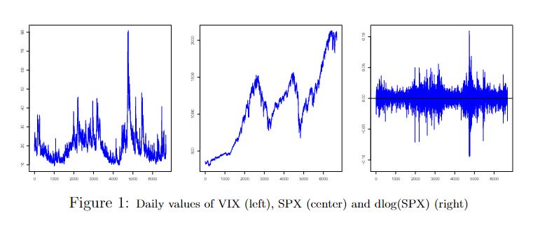
Selected data has been collected from the website of the “Economic Research” department of “St. Louis Fed”. The data set consists of 6679 daily observations of VIX and S&P500 index observed throughout January 1990 to June 2016 period. Manual imputations were performed for a minimal number of non-available data points.

Model design

We compared three models with neural networks as well as VAR and ARIMA models. The response variable is the VIX value. The regressors for our three neural network models are the VIX taken at up to four lags (Vix4), the VIX taken at one lag with the S&P taken at one lag (Vix1_Spx1), and the VIX with up to four lags with the S&P taken at one lag (Vix4_Spx1), respectively. Necessary transformations are performed on the data as explained in the next section.

As for the network architecture, the type of neural networks used for regression are feed-forward neural networks, where inputs are the regressors and the output is the response variable. As we are using R for our assignment, we are constrained by the features of the available packages. We chose the package nnet. The package considers only one hidden layer. The activation function of the hidden units of nnet is a logistic function, and we set the output unit activation function to linear. We want to determine the best number of hidden units for our application and chosen variables.

A number of additional parameters are needed to practically perform a regression with a neural network. In our case, the neural network of the package nnet uses a back-propagation algorithm, and we need to choose a way to stop the iterative training of the network. In general, training for too long can lead to a function that does not generalize well. The nnet package relies on relative or absolute error stopping criteria but we wanted to implement early stopping by use of a validation sample. The validation sample is a subset of the data which is not included in the training set, and the "optimal training" is considered to be reached when the error on the validation sample reaches a minimum. A test set is used to measure the performance of the network and evaluate its ability to generalize to new data.

Unfortunately, the nnet function does not report the weight parameter estimates for each intermediate iteration, so we had to implement a work-around, fairly expensive in computing time. It proceeds as follows: a network is trained until a given iteration i, results are recorded, then the same network is retrained from scratch until the iteration i+1. We start this process from one, and repeat until a maximum number of iterations chosen arbitrarily is covered. The same initial random seed is used for each loop so that the intermediary results remain the same across all training runs. Our program then automatically selects the weight parameters estimates from the iteration with the minimum validation error.

Neural networks of the back-propagation type can converge to local minima. The back-propagation algorithm starts with random weights and we used those provided by the machinery of the nnet function. But to avoid falling into bad local minima, we allowed for several repeated training runs of the same network, with different initial random seeds.

As we shall see, the results are actually extremely sensitive to initial conditions. Therefore we also included several runs for the sampling procedure of the validation samples.

Since the time series shows clustered volatility, the choice of a particular part of the time series for training heavily impacts the ability to predict on another part. So we used a rolling window for training and sampling observations, all the data outside the window are used for the test set. By averaging the performance over the windows and random seeds for data sampling and network optimization, we hoped to level out issues related to initial conditions.

Performance is evaluated by comparing the mean squared error (MSE) on the test sets.

Model implementation and processing

For the neural network models, the daily data of the VIX are standardized : mean centered and scaled by their standard deviation. The S&P data are taken in differences of log values, and also standardized. The number of training data is 6674.

The rolling window has 2000 observations, and is shifted by 1000 observations each time, so that we have five windows partially overlapping each other. Twenty percent of the observations of a window are taken as validation set, the remaining 1600 observations are used for training. All observations outside the window are the out-of-sample test set.

In our first set of networks to estimate, training and validation of the five windows are prepared only once for all the networks of the set, due to computing time limitations. The number of hidden neurons, based on several initial trials, were taken from {3, 4, 5, 7, 9, 10, 15}. The maximum number of iterations is set at 150. Due to the work-around, this means that each network is trained 150 times, from 1 to 150 intermediary iterations.

Altogether there are 36 thousand networks to train. The optimal network iteration in terms of validation error is selected for each network. After averaging over the windows and initial conditions, we obtain a list of 24 models and number of hidden units, with their reported mean squared error on the training, validation and test sets. The results are presented in the following Table, sorted with increasing validation MSE.

Results

Neural Networks

If we take the validation error as a criterion to select the most adequate model, we would choose the model Vix4_Spx1 with 10 hidden units, with validation MSE of 2.460, its performance on the test set is 4.102. Of all models actually processed, the Vix4 is the best in terms of average performance on the test set, with a MSE of 3.991.

Looking at the results from a different perspective, we do not recognize a pattern in the figures that supports the choice of a particular model, other than its raw performance in terms of MSE. We would expect that the performance improves with an increasing number of hidden units, then decreases when there are too many. In that case, the minimum validation error would indicate the choice of the number of hidden units. Also, none of the three models dominates another.

Unfortunately, running the same procedure with different random seeds for the sampling, gave fairly different results. The procedure does not give us meaningful results in terms of choice of model or number of hidden units.

The computing time, above one hour for the set of networks we described, does not allow for a large number of different samplings or different initial weights.

Nevertheless, we ran a second set of networks with the hope to discover some consistency in the results. We concentrated our efforts on a set of networks with the model Vix4, number of hidden units considered in {5, 7, 9, 10, 12, 14, 16, 20}, and 4 training schemes with different random seeds (that is, 4 times 5 windows described earlier), for each of the combinations.

After several hours of processing, the results remained disappointing. Averaged over the windows, sampling and initial conditions, the validation error does seem to have a slight decreasing pattern, with a performance spike for 14 hidden units (Figure 2). But in terms of performance on the test sets, 16 hidden units and 9 hidden units are best, with no noticeable trend or curvature. It could be that running the process for a much larger number of initial conditions does show some usable relationship between number of hidden units, but this is not possible to run due to the processing time of our implementation.

If we consider the individual networks, and take the best networks in terms of test MSE for each window (see previous table), we get some interesting results. If we compare the MSE of the neural network with that of the ARIMA model for a same window (i.e. the same test data, so that the MSE is comparable), we see that the neural networks performed slightly better than the ARIMA models, for the two last windows. These are the two windows that contain the very high volatility periods. It seems that the neural networks that were trained in the less volatile part of the time series are not able to generalize well to the highly volatile periods, when compared with the ARIMA models, on the same test data.

Unfortunately, the lowest validation criterion, though useful for early stopping, would not pick up those best models out of the list. Among other reasons, the training and validation samples being different when the sampling seed is different, the MSE cannot be compared.

Illustration for two particular networks

The following figure(left) illustrates the early stopping mechanism. The network is from window 1, with 7 hidden units and test MSE of 6.467. We see that if we didn’t have this approach and took the network estimated at the maximum number of iterations or some relative measure to the training error, we would end up with a model with a much worse error on the test set, indicating a poorer ability to generalize. In addition the figure compares the predicted VIX to the actual VIX. We see that the same illustrated network fails to generalize. Probably because the test data are on a range of values not covered by the training and validation data. On the other hand, a network of window 5 (bottom), stopped at iteration 33, 9 hidden units, with a test MSE of 1.597, performs well: the test data lie in the zone covered by the training and validation data.

VAR and ARIMA models

In parallel with the development of the neural network application, we also applied time series auto-regressive models, so that we could have a benchmark to compare with the neural network application.

Before employing ARIMA model, the stationarity of the time series is checked by the augmented Dickey-Fuller test, which indicates that the first difference of VIX time series is stationary. Based on the PACF plot and because we prefer simpler models, we select the ARIMA(3,1,0). The ARIMA is then re-estimated on each of the the five different training windows and the MSE is calculated on the respective test sets. In case of the ARIMA, there is no validation sample, so all the data of a window are available for estimation.

To consider the potential influence of S&P 500 index, a vector auto-regressive (VAR) model is also then applied. As we are only interested in predicting VIX, non-stationary series in levels can still be used in VAR model. In our case, VIX values and log S&P 500 returns are included in the vector. The auto selection function recommends a VAR(4) model, which is then estimated on each of the five windows, the MSE is calculated on the respective test sets.

The MSEs of ARIMA(3,1,0) on those five test sets are 2.825, 2.614, 2.548, 2.020 and 1.604 respectively. The overall MSE equals to 2.3226. The VAR(4) model provides a slightly lower MSE of 2.3188, so that it does not improve substantially the predictions compared with the ARIMA.

Discussion

The application of neural network did not provide evidence to select a model among the three models proposed. Nor did we have an indication of the best architecture in terms of hidden units. We can say that 150 iterations was generally sufficient to train the networks. Choosing the optimal set of weights for network with the criterion of minimal validation MSE provided a good approach for early stopping.

It might be that more lags are needed, or a transformation of the VIX data, to improve the performance. A larger number of initial conditions for the sampling and for the weights might allow to avoid possible local minima. Cross-validation could be used instead of the one validation set sampling approach.

As for the contribution of S&P, which is fairly correlated with VIX contemporaneously, it might contain little information for the prediction of VIX one day ahead. An indication for this with the traditional models is that the VAR model did not improve the prediction error compared with the ARIMA models.

In some cases, the neural network performed better on the test set than ARIMA model. The poor performance on the other parts of the time series compared to ARIMA is probably due to lack of generalization.

The major obstacle however is the package we used. We had to program ourselves features that are readily available in other applications (such as MatLab), like the early stopping procedure and support for designing the scheme of training, validation and test sets. This led us to implement workarounds that were unnecessarily complex and very programming time and processing time consuming. Processing time was probably over 100 times higher if we had had access to the intermediary results. This limited our exploration of the space of different models, parameters or initial conditions. Also, we had little control over activation functions, optimization algorithms, and of course the basic setting of a feed-forward neural network with the back-propagation algorithm.